6 Stability
Network stability is a key factor in understanding the robustness of ecological systems.
We collected lots of methods to reflect the stability and complexity in MetaNet, these algorithms are coded using Parallel Computing which can be much faster.
6.1 Network construction
It is very important to compare networks stability based on different groups.
For example, we have three groups of samples: NS, WS, CS, n=6 (in real research, n should be bigger for a meaningful result), we can construct three group networks for each group and compare them.
- We can extract three-group sub-nets from the whole network:
# extract three-group sub-nets
hebing(otutab, metadata$Group) -> otutab_G
head(otutab_G)

# whole network
t(otutab) -> totu
c_net_calculate(totu) -> corr
c_net_build(corr, r_threshold = 0.65) -> co_net

group_net_par <- extract_sample_net(co_net, otutab_G, save_net = "../Group_subnet")
group_nets <- readRDS("../Group_subnet.RDS")

names(group_nets)- Or construct a network for each group specifically:
data("otutab", package = "pcutils")

totu <- t(otutab)
# check all rows matched
all(rownames(totu) == rownames(metadata))

# Use RMT threshold or not?
rmt <- FALSE
group_nets <- lapply(levels(metadata$Group), \(i){
  totu[rownames(filter(metadata, Group == !!i)), ] -> t_tmp
  t_tmp[, colSums(t_tmp) > 0] -> t_tmp
  c_net_calculate(t_tmp) -> c_tmp
  if (rmt) {
    RMT_threshold(c_tmp, verbose = F, out_dir = "test/") -> tmp_rmt
    r_thres <- tmp_rmt$r_threshold
  } else {
    r_thres <- 0.6
  }
  c_net_build(c_tmp, r_threshold = r_thres, p_threshold = 0.01, delete_single = T) -> n_tmp
  Abundance_df <- data.frame("Abundance" = colSums(t_tmp))
  c_net_set(n_tmp, Abundance_df, taxonomy %>% select("Phylum"), vertex_class = "Phylum", vertex_size = "Abundance")
})

names(group_nets) <- levels(metadata$Group)
All calculation for network stability provide parallel version, use parallel::detectCores() to get you device cores and set threads >1 to use parallel calculation.
6.2 Robust test
Robust test of networks were done with natural connectivity as it can reflect the stability of networks (1).
Specifically, natural connectivity was calculated after removing the nodes (remove five nodes from a network at one time until 70% of nodes disappear), and the downtrend level of natural connectivity indicated the connectivity performance of the network after being damaged to a certain extent.
# recommend `reps` bigger than 99, you can set `threads >1` to use parallel calculation.
robust_test(group_nets, partial = 0.5, step = 10, reps = 9, threads = 1) -> robust_res
plot(robust_res, mode = 2)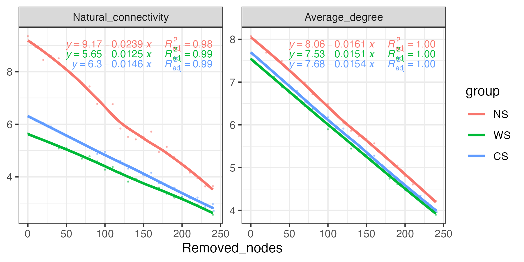
6.3 Community stability
Community stability can be characterized by various indexes, such as robustness, vulnerability and cohesion. Networks with higher robustness and lower vulnerability tend to be more stable (2). Also, community stability is commonly associated with negative interactions, and high percentage of negative correlations within communities is essential for maintaining a stable ecological system.
Robustness
The robustness was regarded as when 50% of nodes were randomly removed and results were based on repetitions of the simulation.
Robustness of a network is defined as the proportion of the remaining nodes in this network after random node removal. For simulations of random nodes removal, a certain proportion of nodes was randomly removed. To test the effects of nodes removal on the remaining nodes, we calculated the abundance-weighted mean interaction strength (wMIS) of node i as follows:
\[ \mathrm{wMIS}_i=\frac{\sum_{j\neq i}b_js_{ij}}{\sum_{j\neq i}b_j} \]
where bj is the relative abundance of species j and sij is the association strength between species i and j, which is measured by Pearson correlation coefficient. Thus, in this study, sij = sji. After removing the selected nodes from the MEN, if wMISi = 0 (all the links to species i have been removed) or wMISi < 0 (not enough mutualistic association between species i and other species for its survival), node i was considered extinct/isolated and thus removed from the network. This process continued until all species had positive wMISs. The proportion of the remaining nodes was reported as the network robustness. We measured the robustness when 50% of random nodes or five module hubs were removed.
# recommend reps bigger than 99, you can set `threads >1` to use parallel calculation.
robustness(group_nets, keystone = F, reps = 99, threads = 1) -> robustness_res
plot(robustness_res, p_value2 = T)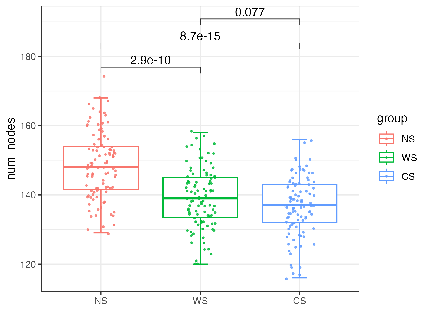
Vulnerability
To evaluate the speed of disturbance spreading within a network, the global efficiency was regarded as the average of the efficiency over all pairs of nodes, which was calculated by the number of edges in the shortest path between paired nodes.
The vulnerability, which reflected the relative contribution of each node to the globe efficiency, was represented by the maximal vulnerability of nodes in the network.
\[ \max\left(\frac{E-E_i}E\right) \]
where E is the global efficiency and Ei is the global efficiency after removing node i and its entire links. The global efficiency of a graph was calculated as the average of the efficiencies over all pairs of nodes:
\[ E=\frac1{n(n-1)}\sum_{i\neq j}\frac1{d(i,j)} \] where d(i, j) is the shortest path length between nodes i and j. The vulnerability was defined as the maximal vulnerability of nodes in the network.
# You can set `threads >1` to use parallel calculation.
vulnerability_res <- vulnerability(group_nets, threads = 1)
plot(vulnerability_res)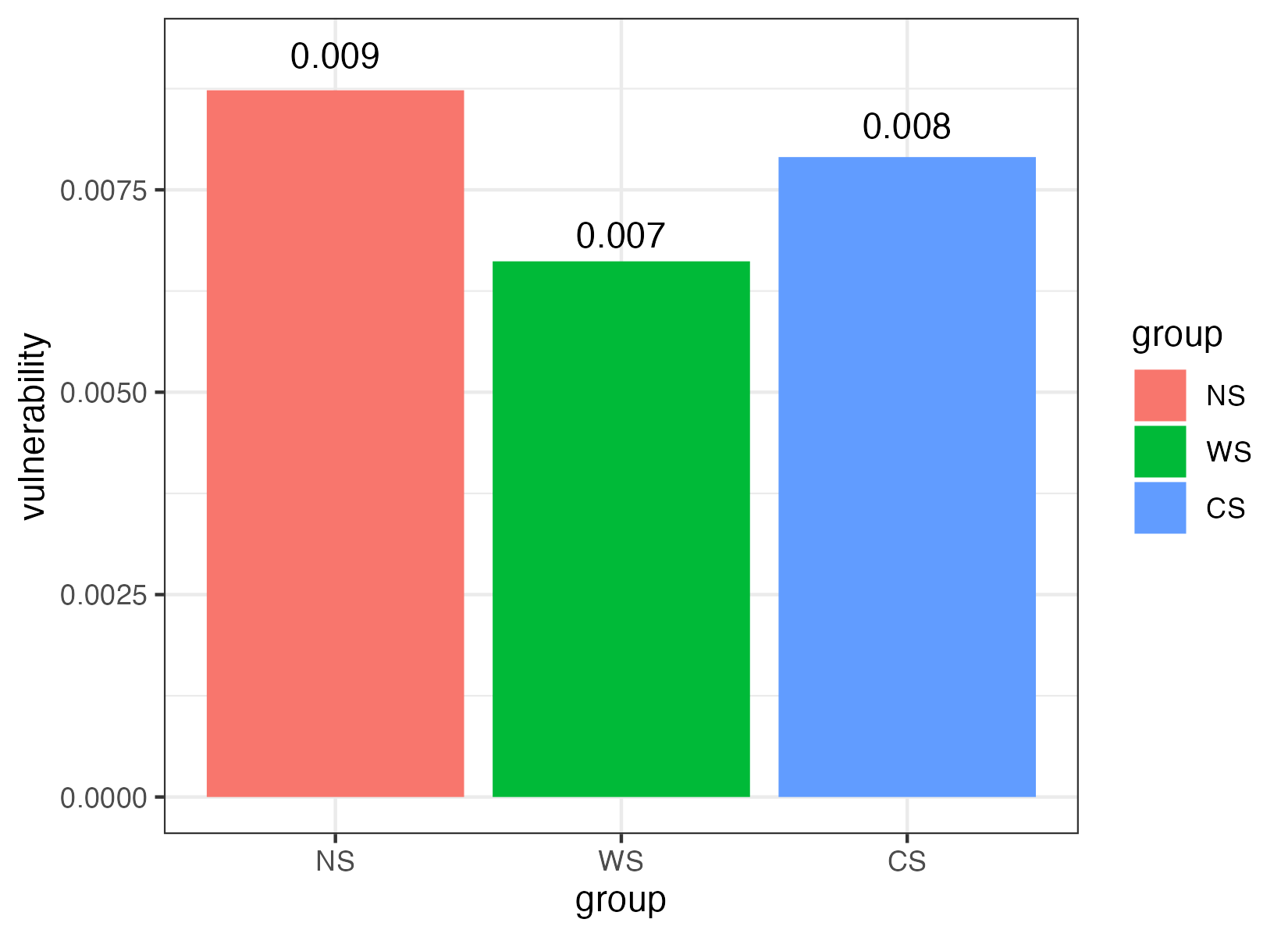
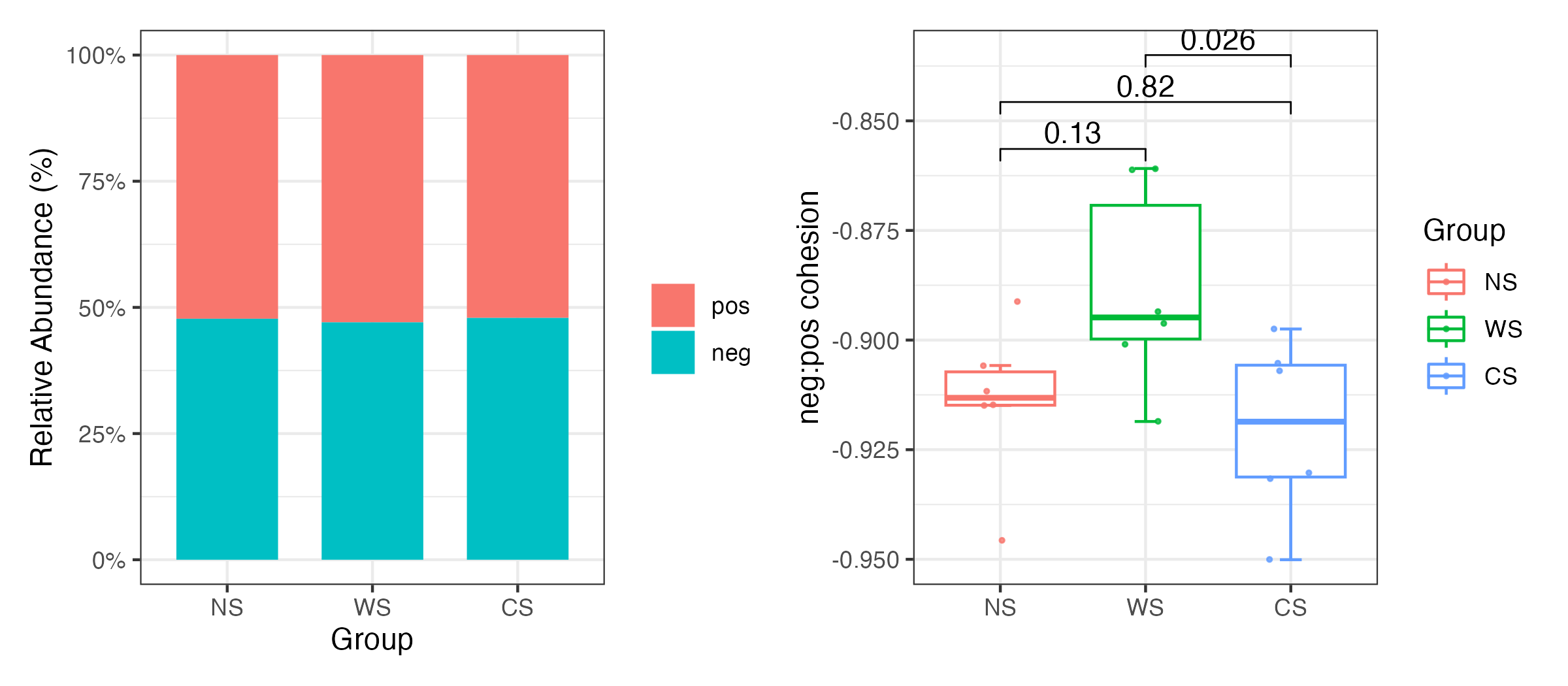
Cohesion
Cohesion was calculated to quantify the connectivity of microbial communities in each group. Cohesion contains both positive and negative cohesion values, which indicate that associations between taxa attributed to positive and negative species interactions as well as similarities and differences in niches of microbial taxa (3).
Briefly, pairwise Pearson correlation matrix across taxa was calculated based on abundance-weighted matrix. After “taxa shuffle” null module-correcting with 200 simulations, average positive and negative correlations was calculated to get a connectedness matrix. Finally, positive and negative cohesions were calculated for each sample respectively by multiplying the abundance-weighted matrix and connectedness matrix. The absolute value of negative: positive cohesion is an important index for community stability.
\[ \text{Cohesion}=\sum_{i=1}^n\text{abundance}_i\times\text{connectednes}s_i \]