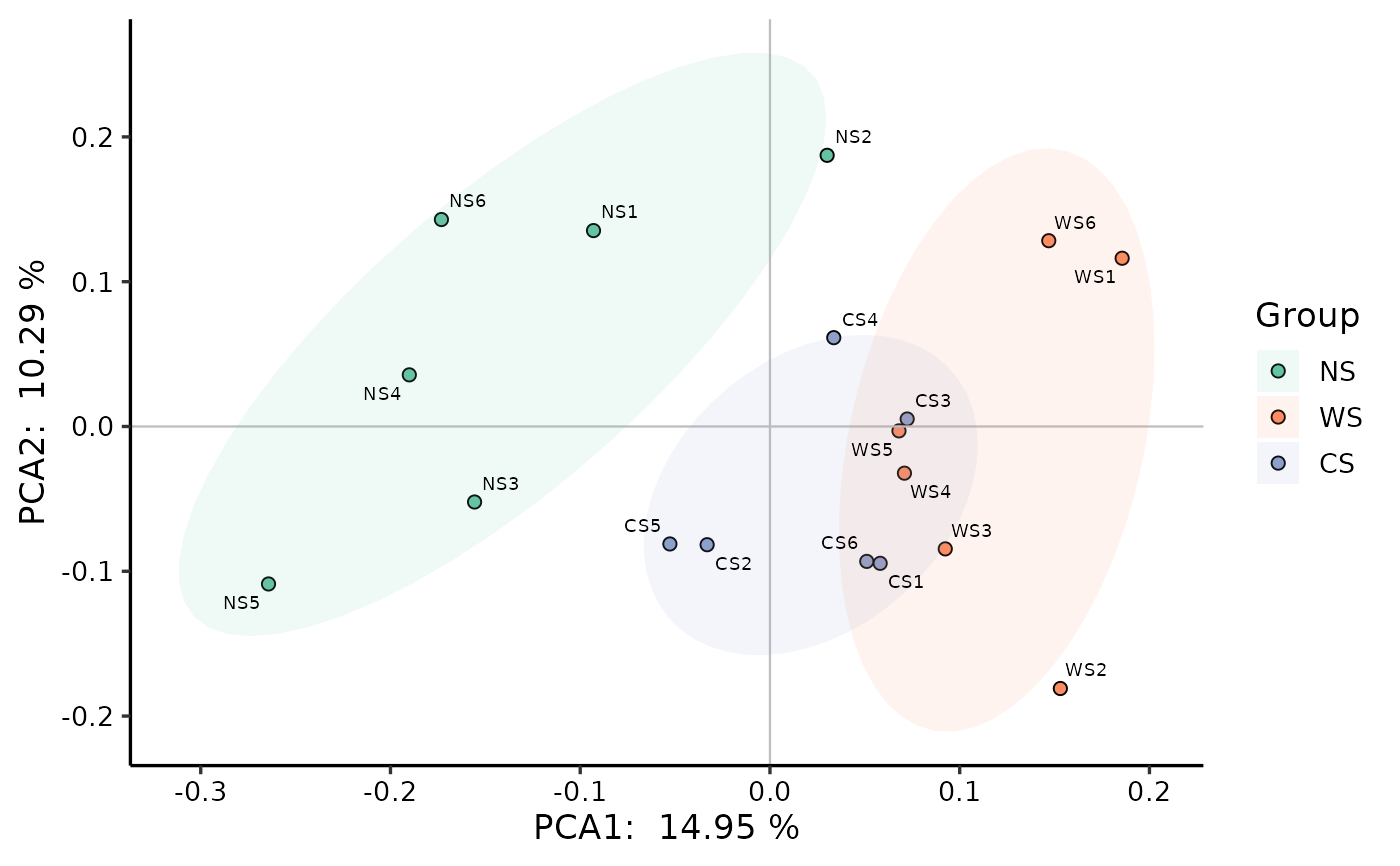
Species abundance data can be preprocessed with Hellinger transformation or chord transformation data before PCA analysis. Because the Hellinger distance or chord distance with-without data is equal to \(\sqrt2\sqrt{1-Ochiai\ similarity}\), therefore, the sorting diagram (type 1 scale) of PCA analysis after Hellinger transformation or chord transformation with-without data is internal sample The distance between the squares is the Ochiai distance. \(\sqrt2\sqrt{1-Ochiai\ similarity}\) is a distance measure, which is also suitable for the analysis of species data. The processed data is then used for pca without norm.
b_analyse(otutab, ...)

# S3 method for class 'data.frame'
b_analyse(
  otutab,
  norm = TRUE,
  method = c("pca"),
  group = NULL,
  dist = "bray",
  ndim = 2,
  scale = FALSE,
  ...
)
Arguments
- otutab
an otutab data.frame, samples are columns, taxs are rows.
- ...
add
- norm
should normalized or not? (hellinger)
- method
one of "pca","pcoa","ca","dca","nmds","plsda","tsne","umap","lda","all"
- group
if needed, give a group vector
- dist
if use pcoa or nmds, your can choose a dist method (default: bray) or input a distance matrix.
- ndim
how many dimension be kept? (default:2). 3 for b_res_3d()
- scale
scale, default: FALSE
Value
b_res object
